This page was generated from doc/code-cells.ipynb. Interactive online version:

Code Cells§

Code, Output, Streams§

An empty code cell:

[ ]:

Two empty lines:

[ ]:

Leading/trailing empty lines:

[1]:



# 2 empty lines before, 1 after

A simple output:

[2]:

6 * 7

[2]:

The standard output stream:

[3]:

print('Hello, world!')

Hello, world!

Normal output + standard output

[4]:

print('Hello, world!')
6 * 7

Hello, world!

[4]:

The standard error stream is highlighted and displayed just below the code cell. The standard output stream comes afterwards (with no special highlighting). Finally, the “normal” output is displayed.

[5]:

import sys

print("I'll appear on the standard error stream", file=sys.stderr)
print("I'll appear on the standard output stream")
"I'm the 'normal' output"

I'll appear on the standard output stream

I'll appear on the standard error stream

[5]:

"I'm the 'normal' output"

Note

Using the IPython kernel, the order is actually mixed up, see https://github.com/ipython/ipykernel/issues/280.

Cell Magics§

IPython can handle code in other languages by means of cell magics:

[6]:

%%bash
for i in 1 2 3
do
    echo $i
done

1
2
3

Special Display Formats§

See IPython example notebook.

Local Image Files§

[7]:

from IPython.display import Image
i = Image(filename='images/notebook_icon.png')
i

[7]:

[8]:

display(i)

Image URLs§

[10]:

Image(url='https://www.python.org/static/img/python-logo-large.png')

[10]:

[11]:

Image(url='https://www.python.org/static/img/python-logo-large.png', embed=True)

[11]:

[12]:

Image(url='https://jupyter.org/assets/homepage/main-logo.svg')

[12]:

Math§

[13]:

from IPython.display import Math
eq = Math(r'\int\limits_{-\infty}^\infty f(x) \delta(x - x_0) dx = f(x_0)')
eq

[13]:

$\displaystyle \int\limits_{-\infty}^\infty f(x) \delta(x - x_0) dx = f(x_0)$

[14]:

display(eq)

$\displaystyle \int\limits_{-\infty}^\infty f(x) \delta(x - x_0) dx = f(x_0)$

[15]:

from IPython.display import Latex
Latex(r'This is a \LaTeX{} equation: $a^2 + b^2 = c^2$')

[15]:

This is a \LaTeX{} equation: $a^2 + b^2 = c^2$

[16]:

%%latex
\begin{equation}
\int\limits_{-\infty}^\infty f(x) \delta(x - x_0) dx = f(x_0)
\end{equation}

\begin{equation} \int\limits_{-\infty}^\infty f(x) \delta(x - x_0) dx = f(x_0) \end{equation}

Plots§

The output formats for Matplotlib plots can be customized via the IPython configuration file ipython_kernel_config.py. This file can be either in the directory where your notebook is located (see the ipython_kernel_config.py in this directory), or in your profile directory (typically ~/.ipython/profile_default/ipython_kernel_config.py). To find out your IPython profile directory, use this command:

python3 -m IPython profile locate

A local ipython_kernel_config.py in the notebook directory also works on https://mybinder.org/. Alternatively, you can create a file with those settings in a file named .ipython/profile_default/ipython_kernel_config.py in your repository.

If you want to use SVG images for Matplotlib plots, add this line to your IPython configuration file:

c.InlineBackend.figure_formats = {'svg'}

If you want SVG images, but also want nice plots when exporting to LaTeX/PDF, you can select:

c.InlineBackend.figure_formats = {'svg', 'pdf'}

If you want to use the default PNG plots or HiDPI plots using 'png2x' (a.k.a. 'retina'), make sure to set this:

c.InlineBackend.rc = {'figure.dpi': 96}

This is needed because the default 'figure.dpi' value of 72 is only valid for the Qt Console.

If you are planning to store your SVG plots as part of your notebooks, you should also have a look at the 'svg.hashsalt' setting.

For more details on these and other settings, have a look at Default Values for Matplotlib’s “inline” Backend.

If you for some reason can’t use a ipython_kernel_config.py file, you can also change these settings with nbsphinx_execute_arguments in your conf.py file:

nbsphinx_execute_arguments = [
    "--InlineBackend.figure_formats={'svg', 'pdf'}",
    "--InlineBackend.rc=figure.dpi=96",
]

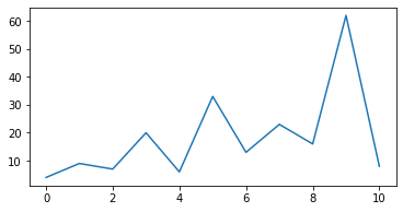
In the following example, nbsphinx should use an SVG image in the HTML output and a PDF image for LaTeX/PDF output.

[17]:

import matplotlib.pyplot as plt

[18]:

fig, ax = plt.subplots(figsize=[6, 3])
ax.plot([4, 9, 7, 20, 6, 33, 13, 23, 16, 62, 8]);

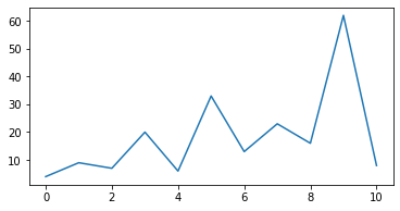
Alternatively, the figure format(s) can also be chosen directly in the notebook (which overrides the setting in nbsphinx_execute_arguments and in the IPython configuration):

[19]:

%config InlineBackend.figure_formats = ['png']

[20]:

fig

[20]:

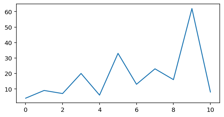
If you want to use PNG images, but with HiDPI resolution, use the special 'png2x' (a.k.a. 'retina') format (which also looks nice in the LaTeX output):

[21]:

%config InlineBackend.figure_formats = ['png2x']

[22]:

fig

[22]:

Pandas Dataframes§

Pandas dataframes should be displayed as nicely formatted HTML tables (if you are using HTML output).

[23]:

import numpy as np
import pandas as pd

[24]:

df = pd.DataFrame(np.random.randint(0, 100, size=[5, 4]),
                  columns=['a', 'b', 'c', 'd'])
df

[24]:

	a	b	c	d
0	36	26	9	75
1	43	18	79	76
2	23	49	21	20
3	17	85	24	94
4	89	79	61	68

For LaTeX output, however, the plain text output is used by default.

To get nice LaTeX tables, a few settings have to be changed:

[25]:

pd.set_option('display.latex.repr', True)

This is not enabled by default because of Pandas issue #12182.

The generated LaTeX tables utilize the booktabs package, so you have to make sure that package is loaded in the preamble with:

\usepackage{booktabs}

In order to allow page breaks within tables, you should use:

[26]:

pd.set_option('display.latex.longtable', True)

The longtable package is already used by Sphinx, so you don’t have to manually load it in the preamble.

Finally, if you want to use LaTeX math expressions in your dataframe, you’ll have to disable escaping:

[27]:

pd.set_option('display.latex.escape', False)

The above settings should have no influence on the HTML output, but the LaTeX output should now look nicer:

[28]:

df = pd.DataFrame(np.random.randint(0, 100, size=[10, 4]),
                  columns=[r'$\alpha$', r'$\beta$', r'$\gamma$', r'$\delta$'])
df

[28]:

	$\alpha$	$\beta$	$\gamma$	$\delta$
0	13	62	67	32
1	53	64	27	87
2	0	33	36	53
3	35	55	45	2
4	1	99	14	51
5	65	83	42	12
6	2	14	43	10
7	36	44	88	4
8	86	40	1	89
9	46	38	69	21

Markdown Content§

[29]:

from IPython.display import Markdown

[30]:

md = Markdown("""
# Markdown

It *should* show up as **formatted** text
with things like [links] and images.

[links]: https://jupyter.org/

![Jupyter notebook icon](images/notebook_icon.png)

## Markdown Extensions

There might also be mathematical equations like
$a^2 + b^2 = c^2$
and even tables:

A     | B     | A and B
------|-------|--------
False | False | False
True  | False | False
False | True  | False
True  | True  | True

""")
md

[30]:

Markdown§

It should show up as formatted text with things like links and images.

Jupyter notebook icon

Markdown Extensions§

There might also be mathematical equations like $a^2 + b^2 = c^2$ and even tables:

A	B	A and B
False	False	False
True	False	False
False	True	False
True	True	True

YouTube Videos§

[31]:

from IPython.display import YouTubeVideo
YouTubeVideo('9_OIs49m56E')

[31]:

Interactive Widgets (HTML only)§

The basic widget infrastructure is provided by the ipywidgets module. More advanced widgets are available in separate packages, see for example https://jupyter.org/widgets.

The JavaScript code which is needed to display Jupyter widgets is loaded automatically (using RequireJS). If you want to use non-default URLs or local files, you can use the nbsphinx_widgets_path and nbsphinx_requirejs_path settings.

[32]:

import ipywidgets as w

[33]:

slider = w.IntSlider()
slider.value = 42
slider

A widget typically consists of a so-called “model” and a “view” into that model.

If you display a widget multiple times, all instances act as a “view” into the same “model”. That means that their state is synchronized. You can move either one of these sliders to try this out:

[34]:

slider

You can also link different widgets.

Widgets can be linked via the kernel (which of course only works while a kernel is running) or directly in the client (which even works in the rendered HTML pages).

Widgets can be linked uni- or bi-directionally.

Examples for all 4 combinations are shown here:

[35]:

link = w.IntSlider(description='link')
w.link((slider, 'value'), (link, 'value'))
jslink = w.IntSlider(description='jslink')
w.jslink((slider, 'value'), (jslink, 'value'))
dlink = w.IntSlider(description='dlink')
w.dlink((slider, 'value'), (dlink, 'value'))
jsdlink = w.IntSlider(description='jsdlink')
w.jsdlink((slider, 'value'), (jsdlink, 'value'))
w.VBox([link, jslink, dlink, jsdlink])

[36]:

tabs = w.Tab()
for idx, obj in enumerate([df, fig, eq, i, md, slider]):
    out = w.Output()
    with out:
        display(obj)
    tabs.children += out,
    tabs.set_title(idx, obj.__class__.__name__)
tabs

Other Languages

The examples shown here are using Python, but the widget technology can also be used with different Jupyter kernels (i.e. with different programming languages).

Troubleshooting§

To obtain more information if widgets are not displayed as expected, you will need to look at the error message in the web browser console.

To figure out how to open the web browser console, you may look at the web browser documentation:

Chrome: https://developer.chrome.com/docs/devtools/open/#console

Firefox: https://developer.mozilla.org/en-US/docs/Tools/Web_Console#opening-the-web-console

The error is most probably linked to the JavaScript files not being loaded or loaded in the wrong order within the HTML file. To analyze the error, you can inspect the HTML file within the web browser (e.g.: right-click on the page and select View Page Source) and look at the <head> section of the page. That section should contain some JavaScript libraries. Those relevant for widgets are:

<!-- require.js is a mandatory dependency for jupyter-widgets -->
<script crossorigin="anonymous" integrity="sha256-Ae2Vz/4ePdIu6ZyI/5ZGsYnb+m0JlOmKPjt6XZ9JJkA=" src="https://cdnjs.cloudflare.com/ajax/libs/require.js/2.3.4/require.min.js"></script>
<!-- jupyter-widgets JavaScript -->
<script type="text/javascript" src="https://unpkg.com/@jupyter-widgets/html-manager@^0.18.0/dist/embed-amd.js"></script>
<!-- JavaScript containing custom Jupyter widgets -->
<script src="../_static/embed-widgets.js"></script>

The two first elements are mandatory. The third one is required only if you designed your own widgets but did not publish them on npm.js.

If those libraries appear in a different order, the widgets won’t be displayed.

Here is a list of possible solutions:

If the widgets are not displayed, see #519.
If the widgets are displayed multiple times, see #378.

Arbitrary JavaScript Output (HTML only)§

[37]:

%%javascript

var text = document.createTextNode("Hello, I was generated with JavaScript!");
// Content appended to "element" will be visible in the output area:
element.appendChild(text);

Unsupported Output Types§

If a code cell produces data with an unsupported MIME type, the Jupyter Notebook doesn’t generate any output. nbsphinx, however, shows a warning message.

[38]:

display({
    'text/x-python': 'print("Hello, world!")',
    'text/x-haskell': 'main = putStrLn "Hello, world!"',
}, raw=True)

Data type cannot be displayed: text/x-python, text/x-haskell

ANSI Colors§

The standard output and standard error streams may contain ANSI escape sequences to change the text and background colors.

[39]:

print('BEWARE: \x1b[1;33;41mugly colors\x1b[m!', file=sys.stderr)
print('AB\x1b[43mCD\x1b[35mEF\x1b[1mGH\x1b[4mIJ\x1b[7m'
      'KL\x1b[49mMN\x1b[39mOP\x1b[22mQR\x1b[24mST\x1b[27mUV')

ABCDEFGHIJKLMNOPQRSTUV

BEWARE: ugly colors!

The following code showing the 8 basic ANSI colors is based on https://tldp.org/HOWTO/Bash-Prompt-HOWTO/x329.html. Each of the 8 colors has an “intense” variation, which is used for bold text.

[40]:

text = ' XYZ '
formatstring = '\x1b[{}m' + text + '\x1b[m'

print(' ' * 6 + ' ' * len(text) +
      ''.join('{:^{}}'.format(bg, len(text)) for bg in range(40, 48)))
for fg in range(30, 38):
    for bold in False, True:
        fg_code = ('1;' if bold else '') + str(fg)
        print(' {:>4} '.format(fg_code) + formatstring.format(fg_code) +
              ''.join(formatstring.format(fg_code + ';' + str(bg))
                      for bg in range(40, 48)))

            40   41   42   43   44   45   46   47
   30  XYZ  XYZ  XYZ  XYZ  XYZ  XYZ  XYZ  XYZ  XYZ 
 1;30  XYZ  XYZ  XYZ  XYZ  XYZ  XYZ  XYZ  XYZ  XYZ 
   31  XYZ  XYZ  XYZ  XYZ  XYZ  XYZ  XYZ  XYZ  XYZ 
 1;31  XYZ  XYZ  XYZ  XYZ  XYZ  XYZ  XYZ  XYZ  XYZ 
   32  XYZ  XYZ  XYZ  XYZ  XYZ  XYZ  XYZ  XYZ  XYZ 
 1;32  XYZ  XYZ  XYZ  XYZ  XYZ  XYZ  XYZ  XYZ  XYZ 
   33  XYZ  XYZ  XYZ  XYZ  XYZ  XYZ  XYZ  XYZ  XYZ 
 1;33  XYZ  XYZ  XYZ  XYZ  XYZ  XYZ  XYZ  XYZ  XYZ 
   34  XYZ  XYZ  XYZ  XYZ  XYZ  XYZ  XYZ  XYZ  XYZ 
 1;34  XYZ  XYZ  XYZ  XYZ  XYZ  XYZ  XYZ  XYZ  XYZ 
   35  XYZ  XYZ  XYZ  XYZ  XYZ  XYZ  XYZ  XYZ  XYZ 
 1;35  XYZ  XYZ  XYZ  XYZ  XYZ  XYZ  XYZ  XYZ  XYZ 
   36  XYZ  XYZ  XYZ  XYZ  XYZ  XYZ  XYZ  XYZ  XYZ 
 1;36  XYZ  XYZ  XYZ  XYZ  XYZ  XYZ  XYZ  XYZ  XYZ 
   37  XYZ  XYZ  XYZ  XYZ  XYZ  XYZ  XYZ  XYZ  XYZ 
 1;37  XYZ  XYZ  XYZ  XYZ  XYZ  XYZ  XYZ  XYZ  XYZ

ANSI also supports a set of 256 indexed colors. The following code showing all of them is based on http://bitmote.com/index.php?post/2012/11/19/Using-ANSI-Color-Codes-to-Colorize-Your-Bash-Prompt-on-Linux.

[41]:

formatstring = '\x1b[38;5;{0};48;5;{0}mX\x1b[1mX\x1b[m'

print('  + ' + ''.join('{:2}'.format(i) for i in range(36)))
print('  0 ' + ''.join(formatstring.format(i) for i in range(16)))
for i in range(7):
    i = i * 36 + 16
    print('{:3} '.format(i) + ''.join(formatstring.format(i + j)
                                      for j in range(36) if i + j < 256))

  +  0 1 2 3 4 5 6 7 8 91011121314151617181920212223242526272829303132333435
  0 XXXXXXXXXXXXXXXXXXXXXXXXXXXXXXXX
 16 XXXXXXXXXXXXXXXXXXXXXXXXXXXXXXXXXXXXXXXXXXXXXXXXXXXXXXXXXXXXXXXXXXXXXXXX
 52 XXXXXXXXXXXXXXXXXXXXXXXXXXXXXXXXXXXXXXXXXXXXXXXXXXXXXXXXXXXXXXXXXXXXXXXX
 88 XXXXXXXXXXXXXXXXXXXXXXXXXXXXXXXXXXXXXXXXXXXXXXXXXXXXXXXXXXXXXXXXXXXXXXXX
124 XXXXXXXXXXXXXXXXXXXXXXXXXXXXXXXXXXXXXXXXXXXXXXXXXXXXXXXXXXXXXXXXXXXXXXXX
160 XXXXXXXXXXXXXXXXXXXXXXXXXXXXXXXXXXXXXXXXXXXXXXXXXXXXXXXXXXXXXXXXXXXXXXXX
196 XXXXXXXXXXXXXXXXXXXXXXXXXXXXXXXXXXXXXXXXXXXXXXXXXXXXXXXXXXXXXXXXXXXXXXXX
232 XXXXXXXXXXXXXXXXXXXXXXXXXXXXXXXXXXXXXXXXXXXXXXXX

You can even use 24-bit RGB colors:

[42]:

start = 255, 0, 0
end = 0, 0, 255
length = 79
out = []

for i in range(length):
    rgb = [start[c] + int(i * (end[c] - start[c]) / length) for c in range(3)]
    out.append('\x1b['
               '38;2;{rgb[2]};{rgb[1]};{rgb[0]};'
               '48;2;{rgb[0]};{rgb[1]};{rgb[2]}mX\x1b[m'.format(rgb=rgb))
print(''.join(out))

XXXXXXXXXXXXXXXXXXXXXXXXXXXXXXXXXXXXXXXXXXXXXXXXXXXXXXXXXXXXXXXXXXXXXXXXXXXXXXX

	$\alpha$	$\beta$	$\gamma$	$\delta$
0	13	62	67	32
1	53	64	27	87
2	0	33	36	53
3	35	55	45	2
4	1	99	14	51
5	65	83	42	12
6	2	14	43	10
7	36	44	88	4
8	86	40	1	89
9	46	38	69	21

	$\alpha$	$\beta$	$\gamma$	$\delta$
0	13	62	67	32
1	53	64	27	87
2	0	33	36	53
3	35	55	45	2
4	1	99	14	51
5	65	83	42	12
6	2	14	43	10
7	36	44	88	4
8	86	40	1	89
9	46	38	69	21

	$\alpha$	$\beta$	$\gamma$	$\delta$
0	13	62	67	32
1	53	64	27	87
2	0	33	36	53
3	35	55	45	2
4	1	99	14	51
5	65	83	42	12
6	2	14	43	10
7	36	44	88	4
8	86	40	1	89
9	46	38	69	21